Running KPP

Now that KPP is properly compiled, we proceed to running the first test case to make sure it works! It’s advised to have the official KPP manual along with you during this section.

The first test case

We now follow the manual and begin running the Chapman stratospheric mechanism as a test case. This will allow us to illustrate some key features when running KPP.

In order to run a simulation on KPP, it needs three things:

• a .kpp file (type ls $KPP_HOME/examples to see some examples of those)
• a .spc file (type ls $KPP_HOME/models to see some examples of those)
• a .eqn file (type ls $KPP_HOME/models to see some examples of those)

We begin by creating a directory to run this first test. Let’s call this directory test1. We can create this directory anywhere: even inside KPP’s home directory, although, for the sake of simplicity, let’s create it in your home directory:

cd $HOME
mkdir test1

Now let’s go to that directory with cd test1. Following the manual, let us create a file called small_strato.kpp with the following contents:

#MODEL      small_strato
#LANGUAGE   Fortran90
#INTEGRATOR rosenbrock
#DRIVER     general

You can do this by typing notepad++ small_strato.kpp in the test1 directory, if using Notepad++, or by using another editor of your choice (replace notepad++ with gedit for example). Then just paste the content above in the file, save and exit it.

This file tells KPP what model to use (small_strato.def) and how to process it (most importantly for us here, it tells KPP to generate a Fortran 90 code, although it can also generate C and Matlab code). Many other options can be added to this file and you can learn more about them in the KPP manual.

If our changes to .bashrc are correct, then KPP should be able to find the correct model, since the small_strato model (given by small_strato.def) is located in the models directory, in the KPP home directory. We test this by running KPP on our recently created file with

kpp small_strato.kpp

You should see the following lines on your screen:

This is KPP-2.2.3.

KPP is parsing the equation file.
KPP is computing Jacobian sparsity structure.
KPP is starting the code generation.
KPP is initializing the code generation.
KPP is generating the monitor data:
    - small_strato_Monitor
KPP is generating the utility data:
    - small_strato_Util
KPP is generating the global declarations:
    - small_strato_Main
KPP is generating the ODE function:
    - small_strato_Function
KPP is generating the ODE Jacobian:
    - small_strato_Jacobian
    - small_strato_JacobianSP
KPP is generating the linear algebra routines:
    - small_strato_LinearAlgebra
KPP is generating the Hessian:
    - small_strato_Hessian
    - small_strato_HessianSP
KPP is generating the utility functions:
    - small_strato_Util
KPP is generating the rate laws:
    - small_strato_Rates
KPP is generating the parameters:
    - small_strato_Parameters
KPP is generating the global data:
    - small_strato_Global
KPP is generating the stoichiometric description files:
    - small_strato_Stoichiom
    - small_strato_StoichiomSP
KPP is generating the driver from none.f90:
    - small_strato_Main
KPP is starting the code post-processing.

KPP has succesfully created the model "small_strato".

Note

If you get an error message here, go back a few steps and make sure the $KPP_HOME and the $PATH variable are set correctly, and be sure that both KPP can be found and the correct model files small_strato are in $KPP_HOME/models.

If indeed you see this output (or something very similar) it means you were successful in creating the model. Now if you list your files with the ls command, you’ll see many new files:

Makefile_small_strato           small_strato.map
small_strato_Function.f90       small_strato_mex_Fun.f90
small_strato_Global.f90         small_strato_mex_Hessian.f90
small_strato_Hessian.f90        small_strato_mex_Jac_SP.f90
small_strato_HessianSP.f90      small_strato_Model.f90
small_strato_Initialize.f90     small_strato_Monitor.f90
small_strato_Integrator.f90     small_strato_Parameters.f90
small_strato_Jacobian.f90       small_strato_Precision.f90
small_strato_JacobianSP.f90     small_strato_Rates.f90
small_strato.kpp                small_strato_Stoichiom.f90
small_strato_LinearAlgebra.f90  small_strato_StoichiomSP.f90
small_strato_Main.f90           small_strato_Util.f90

Most of them end with a .f90 extension, which tells us they are Fortran 90 codes. These codes have to be compiled into an executable file which is what will actually process and run the kinetic model. So the next step is to compile every one of those code together into one executable and run it. To do that, let’s focus for now on the Makefile_small_strato. This is a text file that tells your computer which Fortran compiler to use to compile, which files to use, etc. We need to modify it, so open the Makefile_small_strato file (again using your preferred editor) and find where it says

#COMPILER = G95
#COMPILER = LAHEY
COMPILER = INTEL
#COMPILER = PGF
#COMPILER = HPUX
#COMPILER = GFORTRAN

Each of the lines is a different Fortran compiler, and your computer is only going to see the line that doesn’t start with a # (we say that the lines with # are commented and therefore the computer doesn’t “see” them). So, currently, these lines are telling the computer to use the Intel Fortran compiler, ifort.

If you are using ifort, you should leave it as it is. However, ifort is paid, so chances are you are using another compiler. If this is the case, put the # in front of the INTEL options and take it out of the line which has the name of your compiler. If you don’t know which compiler you have, chances are you have gfortran, which is free and the one we will use here. You can install gfortran with sudo apt install gfortran (or the equivalent installation command for your system). So, for gfortran, you should make the above lines of code look like the following:

#COMPILER = G95
#COMPILER = LAHEY
#COMPILER = INTEL
#COMPILER = PGF
#COMPILER = HPUX
COMPILER = GFORTRAN

When doing that we say that we “uncommented” the gfortran line, since every line that starts with a # is commented and not read by the system. You can save and exit the file.

Now all you have to do is run the following command:

make -f Makefile_small_strato which will compile your Fortran code into an

executable file (.exe) using the options we just set. You should see a lot of lines appearing on screen starting with gfortran, maybe some warnings, and if no error messages appear the compilation was successful.

Now you’ll see many more new files, including one called small_strato.exe, which is your executable file (run ls again list everything and see that). This is the executable that will actually calculate the concentrations using the model.

To test if it works, run the following command:

./small_strato.exe

which will run the executable. You should see some output on the screen with concentrations, like Fig. Output concentrations of the first test case.

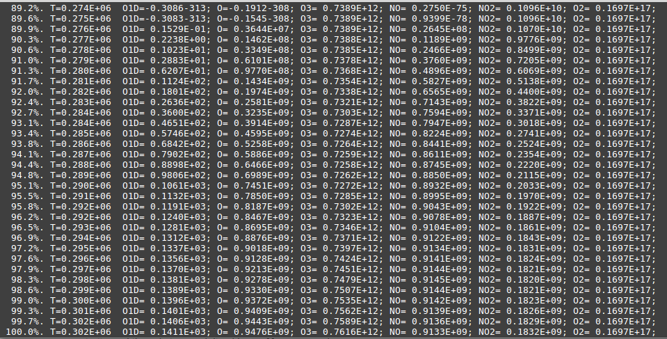
Output concentrations of the first test case.

If this is the case, then your run was successful and everything worked well! You just calculated the concentrations of the compounds in the small_strato model with the pre-defined initial conditions.

Understanding the test case

Now let’s understand why our run of small_strato.exe was successful and what happened. First, by running kpp small_strato, what we did was to tell KPP to open a file called small_strato.kpp, in the current directory and do what that file tells it to do. In the first line of the file there is the command

#MODEL      small_strato

which tells KPP to look for a file called small_strato.def. Since the file is in KPP’s models directory (at $HOME_KPP/models), KPP had no problems finding it. This file has the initial concentrations you want to use in the model, the time step, etc. It also links two other files (small_strato.spc and small_strato.eqn), which tell KPP with chemical species and chemical equations to use (effectively defining the mechanism).

After receiving all that information, KPP finally creates a Fortran 90 code (because it says so in the small_strato.kpp we created) with our small stratospheric model containing our pre-defined initial conditions, time step, chemical reactions and so on.

The code, however, has to be compiled before run, so that is why we issued the command make, which compiles the code according to the file Makefile_small_strato (which is where we specified the Fortran compiler). This step creates an executable file, which has the extension .exe and is ready to be run. By running the .exe file we ran a program that got our initial concentrations of the species we defined and, based on the chemical reactions, calculated, step by step, their concentrations in each time step.

At each step, the model is not only printing the concentrations on screen, but it is also writing them into a file called small_strato.dat, which is a column-separated text file. This file can be used to see, plot, make calculations with the data and so on. However, you should be careful because the order of the concentrations that appear on screen isn’t the same order KPP uses for the .dat file. You can learn about the ordering at page 7 of the KPP manual, but a good rule of thumb is to check the file with a .map extension (in this case, small_strato.map) and take a look at the species section. The file output order is the ordering of the variable species followed by the species on the fixed species.

In the case of small_strato the order printed on the file (you can check it on small_strato.map) is

time, O1D, O, O3, NO, NO2, M, O2

The time is always going to be the first column, and it is always going to be in hours since the start of the simulation. Since the solar forcing matters here, we need to keep track of the time of day that the simulation started. In this case it was at noon, because that’s the way the .def file is set (we will talk about this in more detail in the sections to come).

We can read that data in many ways. I present below a quick python script to plot the concentrations as a function of the hour of the day

import pandas as pd
from matplotlib import pyplot as plt
concs = pd.read_csv('small_strato.dat', index_col=0, delim_whitespace=True, header=None).apply(pd.to_numeric, errors='coerce')
concs.columns = ['O1D', 'O', 'O3', 'NO', 'NO2', 'M', 'O2']
concs.index.name = 'Hours since noon'
concs.plot(ylim=[1.e8, None], logy=True, y=['O3', 'NO', 'NO2'], grid=True)
plt.savefig('test1_time.png')

Note

KPP has a small issue with formatting and sometimes prints a number that can’t be read because some strings are missing. For example, printing 3.4562-313. This can’t be normally read and it’s supposed to be 3.4562E-313 and this (apparently) only happens when the number is close to machine-precision (which we would interpret as zero). The program above takes this issue into consideration (in line 3) when reading the file, but you should pay attention to that when trying to read with by other means.

If you have ever seen python before, this code should be pretty intuitive. If you haven’t you can still use it easily (depending on how you got python, you might have to install python’s pandas package). This code generates the following plot of the concentrations:

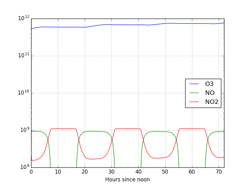
We can see that the NOx concentrations follow the solar cycle, which is indicative that the model is indeed working properly. However we see that the O3 concentrations still haven’t stabilized. This tells us that we need to run the model for longer. Let us take this chance to modify the small_strato example a bit, try and make the O3 concentrations stabilize and learn how to alter/create models.