Modifying and improving the example

Increasing the length of the simulation

There are two ways to make modifications on the model. The first, which works for simple changes, is to modify the Fortran code itself. The second is to change the KPP model itself (the .def files etc.) before it gets compiled. This latter method is more general, so this is the one we will focus on this guide. Since all we want for now is to increase the total time, we will base ourselves in the original small_strato model and only modify this parameter.

First, create another directory (anywhere you want) called test2 (with mkdir test2) and enter it (with cd test2). Now create a file called my_strato.kpp (with notepad++ my_strato.kpp or gedit my_strato.kpp or whichever text editor you ended up using) and paste the following lines in the file:

#MODEL      my_strato
#LANGUAGE   Fortran90
#INTEGRATOR rosenbrock
#DRIVER     general

At this point if you run kpp my_strato.kpp you should get an error saying "Fatal error : my_strato.def: Can't read file". Which appears because we instructed KPP to search for the file my_strato.def, which doesn’t exist anywhere. So we first must create the my_strato.def file, which ultimately defines the my_strato model.

Let us define our model based on small_strato, since for now all we want to do is to modify the time length of the simulation. In order to preserve the original small_strato.def we’ll copy it and call it my_strato.def, this way we can do any modification on my_strato and the original small_strato will be safe. You can copy the file from the models directory into our working directory (test2) by issuing the following command:

cp $KPP_HOME/models/small_strato.def my_strato.def

Note

When we run KPP from any directory (say, test2), KPP will first look for the files in the current directory and then in its home directory. So can either put our model files in our KPP “models” directory or in our current directory. In this guide we’ll always prefer to keep the model we create/modify in the current directory.

Now you should open the file we just created (for example with notepad++) and find the lines that look like:

#INLINE F90_INIT
        TSTART = (12*3600)
        TEND = TSTART + (3*24*3600)
        DT = 0.25*3600
        TEMP = 270
#ENDINLINE

These are the lines that define the start, end, time step and global temperature of the model. For now, we’ll change only the end time. Notice that they are given in seconds. For example, 3*24*3600 is the amount of seconds in 3 days, meaning that at the moment the simulation is set to run for 3 days, which we saw is not enough. Let us then replace 3 with 30, meaning we will run it for 30 days, to be sure that equilibrium is reached. Now that line should read TEND = TSTART + (30*24*3600). Please also note that TSTART is set to 12*3600, or 12 hours, which means that the starting time of the simulation is at noon.

After this small change we are ready to test run the model. Run kpp my_strato.kpp, which should end with a succesfully created the model message. Now, just like with the previous example, open again the file Makefile_my_strato and uncomment the line that says COMPILER = GFORTRAN, so we can use gfortran instead of Intel. After this is done compile the model with:

make -f Makefile_my_strato

Again, if everything goes well, the my_strato.exe file should be created. You can run ls -tr (which lists every file on your directory ordered by creation time) and see that the last file listed should be the .exe file.

We can now run the model with ./my_strato.exe, which should now take 10 times longer to complete, since we are running it for 10 times as long as before. We can use the Python code given in the last section to read the results. We just need to adjust the name inside the code from small_strato to my_strato.

The plot of the results is

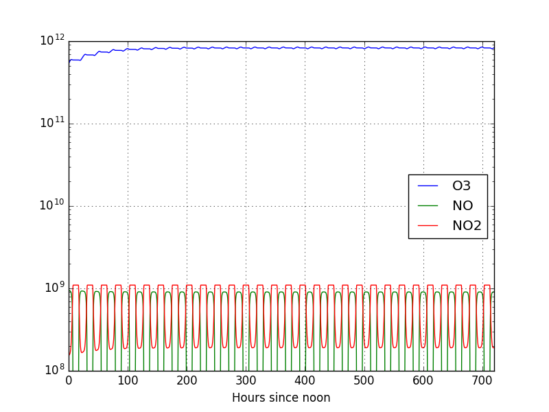
Now we can see that the solution reaches equilibrium after roughly 200 hours. This, however, was only a minor change in the model. Let us now learn how to change some other parameters and examine how the model reacts.

Change in the initial conditions

We try this next change in the same model as before (my_strato). Let’s open my_strato.def and consider an atmosphere with more NO (simulating a more polluted condition). Where it says NO = 8.725E+08;, we make it read NO  = 9.00E+09, which is roughly a 10 times increase in the NO concentration. Let us also change the O3 initial condition and make the O3 line read O3  = 5.00E+10;, simulating an atmosphere that has a lower initial O3 concentration.

Let us also change the line that reads:

#LOOKATALL          {File Output}

We will make it read

#LOOKAT O3; NO; NO2; {File Output}

This latter change makes the program write only time, O3, NO and NO2 into the output file. This simplifies the reading process and saves space, but by doing that we are assuming that we’re not interested in the other species.

Note

This will change the order of the output in the file. But again, checking the .map will give you the correct order. This time you’ll have to consider only the species you specified to be on the output, so, e.g., in this case the order in the .map file is: 1 = O1D, 2 = O, 3 = O3, 4 = NO, 5 = NO2. But since we are writing only O3, NO and NO2, our output file will have the order (time,) O3, NO, NO2 (which are numbers 3, 4, 5, respectively). This will have to be done every time the #LOOKAT parameter is used.

We again go through the same steps: run it with kpp my_strato.kpp, change the compiler to gfortran, compile if with make -f Makefile_my_strato and run it with ./my_strato.exe. This time, since the output file changed, we have to change the code to read it correctly:

import pandas as pd
from matplotlib import pyplot as plt
concs = pd.read_csv('my_strato.dat', index_col=0, delim_whitespace=True, header=None, dtype=None).apply(pd.to_numeric, errors='coerce')
concs.columns = ['O3', 'NO', 'NO2']
concs.index.name = 'Hours since noon'
concs.plot(ylim=[1.e8, None], logy=True, y=['O3', 'NO', 'NO2'], grid=True)
plt.savefig('test21_time.png')

This code produces the following plot:

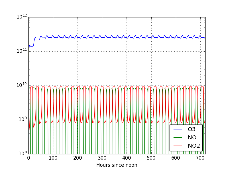
From which we can see that the concentration of ozone stabilized more quickly in this case. As you can see, we can play around with the initial conditions as much as we want and analyse that result of model. In fact, we encourage you to do so. However, let us focus this guide on the next step and modify some more fundamental aspects of the model: the reaction rates.

Modifying the reactions

Now we will alter the reaction rates of some reactions in the model. Keep in mind that these alterations are not meant to be realistic. They are simply done here for the sake of learning how the model works.

Begin again by creating a test3 directory anywhere and going into it (mkdir test3 && cd test3). In this directory, create a file called strato3.kpp with the following contents:

#MODEL      strato3
#LANGUAGE   Fortran90
#INTEGRATOR rosenbrock
#DRIVER     general

This file tells KPP to look for the strato3.def file. So let us create this file by again copying the small_strato.def file to our current working directory. You can do that with:

cp $KPP_HOME/models/small_strato.def strato3.def

Open the file (notepad++ strato3.def) and find the first two lines which originally read

#include small_strato.spc
#include small_strato.eqn

Which still tells KPP to look for the original small_strato model files when defining the species (.spc) and chemical equations (.eqn). You should modify these lines to the following:

#include strato3.spc
#include strato3.eqn

Also, you should do same modification we did in the last example. That is to change the length of the run from 3 to 30 days by modifying the line that reads TEND = TSTART + (3*24*3600) to make it read TEND = TSTART + (30*24*3600), and to change the line that reads #LOOKATALL to #LOOKAT O3; NO; NO2;.

If you try to run KPP now you’ll again get an error because those files still don’t exist. Let’s create them by copying the original small_strato files, which can be done with the following commands:

cp $KPP_HOME/models/small_strato.spc strato3.spc
cp $KPP_HOME/models/small_strato.eqn strato3.eqn

Now if you try running KPP it should work. But this is still not what we want; this is just the small_strato mechanism with another name, so let us move to the actual changes.

If you check the strato3.spc file you’ll see that it only the definitions of the species used, which wouldn’t make much sense to change for now since we’ll be using the same species, so we will leave it how it is. Now we focus on the strato3.eqn file. If you open it you’ll find the following lines:

#EQUATIONS { Small Stratospheric Mechanism }

<R1>  O2   + hv = 2O            : (2.643E-10) * SUN*SUN*SUN;
<R2>  O    + O2 = O3            : (8.018E-17);
<R3>  O3   + hv = O   + O2      : (6.120E-04) * SUN;
<R4>  O    + O3 = 2O2           : (1.576E-15);
<R5>  O3   + hv = O1D + O2      : (1.070E-03) * SUN*SUN;
<R6>  O1D  + M  = O   + M       : (7.110E-11);
<R7>  O1D  + O3 = 2O2           : (1.200E-10);
<R8>  NO   + O3 = NO2 + O2      : (6.062E-15);
<R9>  NO2  + O  = NO  + O2      : (1.069E-11);
<R10> NO2  + hv = NO  + O       : (1.289E-02) * SUN;

Just for the sake of learning, let us change the photolysis rate (last reaction) to make it a lot slower. We will make the last line read:

<R10> NO2  + hv = NO  + O       : (1.289E-06) * SUN;

Note

This is 4 orders of magnitude slower than it previously was and it may not be realistic! We only make this change for the sake of illustration, so that the output change is easier to see.

You can actually change not only the reaction rate for the equation, but also modify the equations itself here and add (or remove) equations. For now we will leave the equations the way they are.

Now we go through the same steps of running kpp strato3.kpp, changing the compiler to gfortran and running make -f Makefile_strato3. If everything goes well, we’ll see the strato3.exe created. After running ./strato3.exe sure enough strato3.dat is created, which we can plot with the same python code from the last example (only changing the name of the file of course):

Note

This process of running KPP, then changing the Makefile, then compiling, etc., is pretty cumbersome and straightforward. So we included a file called updatenrun.sh in the directory test3 that can be found in the github repo. This is a bash script that does these steps automatically. To run it, you enter sh updatenrun.sh modelname. In this case, for example it shoudl be used with sh updatenrun.sh strato3.

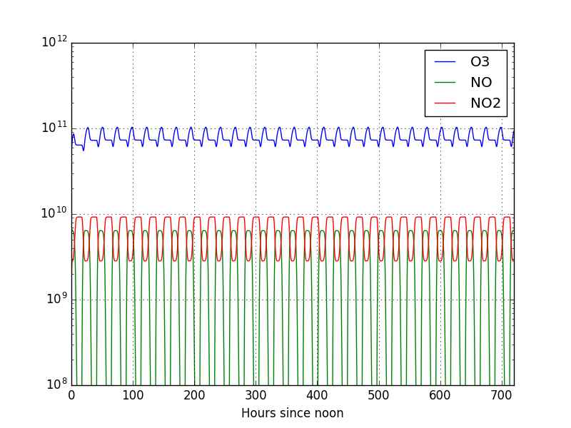
We can see that once again the final result changed. This time, since NO2 is photolizing a lot slower, we see less NO in comparison with the previous plot. We encourage you to try different reaction rates and initial conditions and see what is the result in the model. With the updatenrun.sh script (check the note above) it should be easy!

Now that we have modified the small_strato example in several ways, let take it a step further and create a new model from scratch.

Creating a model from scratch

Now we do one more step and create a completely new model with our own set of reactions. Basically for our new model to be complete we should give it the initial conditions, numerical constraints, species and reactions list. Let us start with the KPP file and move on from there.

We will try to simulate a very small tropospheric model, which we will call ttropo (meaning tiny tropospheric; let’s write it like that just because it’s easier). First let’s create a new directory for our test with mkdir ttropo and move to that new directory with cd ttropo. Now we create the main KPP file with notepad++ ttropo.kpp and put the following lines in it:

#MODEL      ttropo
#LANGUAGE   Fortran90
#INTEGRATOR rosenbrock
#DRIVER     general

Which means tells KPP to look for the ttropo.def file. If you run KPP now it will finish with an error because it won’t find it. But we will create that later. Let us first define our mechanism, i.e., our chemical reactions.

We create the ttropo.eqn file (e.g. with notepad++ ttropo.eqn). Now we will put our reactions in that file, following the syntax that we saw in the previous example. We choose a simplified set of tropospheric reactions that can be written as:

#EQUATIONS { Tiny Tropospheric Mechanism }
<R2>  O    + O2  = O3            : (8.018E-17);
<R1>  NO2  + hv  = NO  + O       : (1.289E-02) * SUN;
<R3>  NO   + O3  = NO2 + O2      : (6.062E-15);
<R41> O3   + hv  = O   + O2      : (5.500E-04) * SUN;
<R42> O3   + hv  = O1D + O2      : (6.000E-05) * SUN*SUN;
<R5>  O1D  + M   = O   + M       : (7.110E-11);
<R6>  O1D + H2O  = 2OH           : (2.2E-10);
<R7>  CO   + OH  = CO2 + HO2     : (2.2E-13);
<R9>  HO2  + NO  = OH  + NO2     : (8.3E-12);
<R10> OH  + NO2  = HNO3          : (1.1E-11);
<R11> HO2 + HO2  = H2O2          : (5.6E-12);
<R12> O3  + HO2  = OH + 2O2      : (2.0E-15);
<R13> H2O2 + hv  = 2OH           : (1.366E-5) * SUN;
<R14> H2O2       = H2O2aq        : (3.3000e-03);
<R15> HNO3       = HNO3aq        : (2.4000e-03);

So copy and paste those lines into ttropo.eqn, save and exit.

Note

Again, some of these reaction constants might not be exactly accurate for tropospheric conditions, so please double-check if you plan on using them for professional means, since the objective here is to only present this as an example.

Now we create the species file, which has to have all the species we used in the reactions above properly defined. We can define a species as being variable (when its concentration can vary according to the kinetics) or fixed (when its concentration is a constant). In this case, we define only M, H2O and O2 as fixed quantities and the other ones as variables:

#include atoms

#DEFVAR
O   = O;            { Oxygen atomic ground state }      
O1D = O;            { Oxygen atomic excited state }
O3  = O + O + O;    { Ozone }
NO2 = N + O + O;    { Nitrogen dioxide }
NO  = N + O;        { Nitric oxide }         
HNO3 = H + N + O+O+O;
H2O2 = H+H + O+O;
CO2  = C + O + O;
CO   = C + O;
OH   = O + H;
HO2  = H + O + O;
H2O2aq = IGNORE;
HNO3aq = IGNORE;

#DEFFIX
M   = O + O + N + N;{ Atmospheric generic molecule }
O2  = O + O;        { Molecular oxygen }
H2O = H + H + O;    { Water }

Again, copy and paste those lines into ttropo.spc, save, exit, and let’s proceed to the .def file. Create ttropo.def with notepad++ ttropo.def. In that file you will write the following lines:

#include ttropo.spc
#include ttropo.eqn

#JACOBIAN SPARSE_LU_ROW      {Use Sparse DATA STRUCTURES}
#DRIVER general
#DOUBLE ON
#STOICMAT ON

#LOOKATALL;                 {File Output}}
#MONITOR O3;N;O;NO;O1D;NO2; {Screen Output}

#CHECK O; N;                   {Check Mass Balance}

#INITVALUES                    {Initial Values}
CFACTOR = 1.    ;              {Conversion Factor}
O3  = 7.65E+11 ; 
NO  = 2.55E+10 ;
NO2 = 0.0E+09 ;
O2  = 1.697E+19 ;
M   = 2.550E+19 ;
H2O = 3.0E+17;
CO  = 2.55E13;

OH     = 0.;
HO2    = 0.;
H2O2   = 0.;
H2O2aq = 0.;
HNO3   = 0.;
HNO3aq = 0.;
O1D    = 0. ;
O      = 0. ;

#INLINE F90_INIT
       TSTART = (12*3600)
       TEND = TSTART + (15*24*3600)
       DT = 0.2*3600
       TEMP = 270
#ENDINLINE

You can see that with this set of definitions we chose to run the model for 15 days, with a time step of 0.2 hours and that many of the initial concentrations are set to zero. Note also that we are again starting the simulation at noon.

With these files we have the complete ttropo model and are ready to run it. We can use the updatenrun.sh script as sh updatenrun.sh ttropo (you’ll have to copy it to the current directory with cp first). It should run successfully now. Note that we again have to check out ttropo.map to find out the order of the species in the output file. We can use the following Python script to plot the results (the correct output order is already included in it):

import pandas as pd
from matplotlib import pyplot as plt

concs = pd.read_csv('ttropo.dat', index_col=0, delim_whitespace=True, header=None, dtype=None).apply(pd.to_numeric, errors='coerce')
concs.columns = ['CO2', 'H2O2aq', 'HNO3aq', 'HNO3', 'H2O2', 'CO', 'O1D', 'O', 'OH', 'HO2', 'O3', 'NO', 'NO2', 'M', 'O2', 'H2O']
concs.index.name = 'Hours since noon'
concs.plot(ylim=[1.e4, None], logy=True, y=['O3', 'NO', 'NO2', 'CO', 'HNO3', 'OH', 'HO2'], grid=True)

plt.savefig('test4_time.png', bbox_inches='tight')
plt.show()

The output of this model can be seen in this figure:

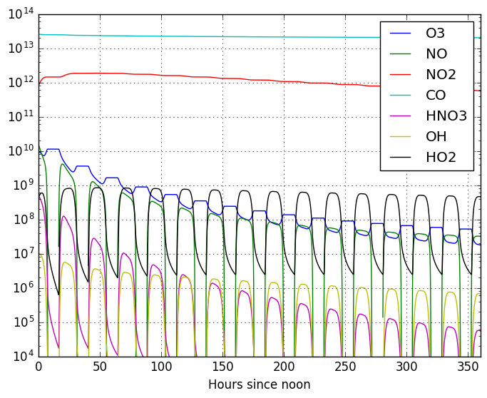
As you can see, in 15 days we ran the model for, it hasn’t reached equilibrium yet. This system of equations will take longer to reach equilibrium state than previous models. You can, once again, investigate the effects of different initial concentrations in the final result, change the reactions and reaction rates, or even fix some quantities in the .spc file.

The creation of any new model from scratch follows the same paths that we just described here. So for other models, following these steps should produce the correct result. For model detailed information not included here, we refer the user to the official manual for KPP.